Is there a way to determine the major orientation of polygon in sf?

Question

I would like to know if there is an off-the-shelf tool or if anyone has developed a method for determining the man axis geographic orientation of spatial shapes. In general, I would like to be able to determine if a shape is oriented east-west or north-south, but ideally there will be an angle or degree measurement associated with each shape.

ArcGIS offers the 'calculate main angle tool' but it is designed for orthogonal shapes and I am working with wildfire perimeters which are blob-like or at least not very orthogonal. At first glance, the Arc tool provides very coarse measurements.

I would like to do this using an sf object, so for an example perhaps use the North Carolina data in the sf package. What is the geographic orientation of each of the 100 counties in North Carolina?

nc <- st_read(system.file("shape/nc.shp", package = "sf"), quiet = TRUE)

Thanks for your help!

Answer 1

THe flightplanning-R package has a function that calculates the minimum bounding rectangle, angle of orientation, height, and width. (https://github.com/caiohamamura/flightplanning-R)

I've adjusted it slightly and used it below in another function to return an sf object with angle of orientation and a POLYGON geometry column. The angle is from 0 (east-west) to 180(also east-west), with 90 being north-south.

# Copied function getMinBBox()
# from https://github.com/caiohamamura/flightplanning-R/blob/master/R/utils.R
# credit there given to: Daniel Wollschlaeger <https://github.com/ramnathv>


library(tidyverse)
library(sf)
library(sfheaders)


nc <- st_read(system.file("shape/nc.shp", package = "sf"), quiet = TRUE) %>%
  st_geometry() %>% st_as_sf()


getMinBBox <- function(x) {
  stopifnot(is.matrix(x), is.numeric(x), nrow(x) >= 2, ncol(x) == 2)
  
  ## rotating calipers algorithm using the convex hull
  H    <- grDevices::chull(x)      ## hull indices, vertices ordered clockwise
  n    <- length(H)      ## number of hull vertices
  hull <- x[H, ]        ## hull vertices
  
  ## unit basis vectors for all subspaces spanned by the hull edges
  hDir  <- diff(rbind(hull, hull[1, ])) ## hull vertices are circular
  hLens <- sqrt(rowSums(hDir^2))        ## length of basis vectors
  huDir <- diag(1/hLens) %*% hDir       ## scaled to unit length
  
  ## unit basis vectors for the orthogonal subspaces
  ## rotation by 90 deg -> y' = x, x' = -y
  ouDir <- cbind(-huDir[ , 2], huDir[ , 1])
  
  ## project hull vertices on the subspaces spanned by the hull edges, and on
  ## the subspaces spanned by their orthogonal complements - in subspace coords
  projMat <- rbind(huDir, ouDir) %*% t(hull)
  
  ## range of projections and corresponding width/height of bounding rectangle
  rangeH  <- matrix(numeric(n*2), ncol=2)  ## hull edge
  rangeO  <- matrix(numeric(n*2), ncol=2)  ## orthogonal subspace
  widths  <- numeric(n)
  heights <- numeric(n)
  
  for(i in seq(along=numeric(n))) {
    rangeH[i, ] <- range(projMat[  i, ])
    
    ## the orthogonal subspace is in the 2nd half of the matrix
    rangeO[i, ] <- range(projMat[n+i, ])
    widths[i]   <- abs(diff(rangeH[i, ]))
    heights[i]  <- abs(diff(rangeO[i, ]))
  }
  
  ## extreme projections for min-area rect in subspace coordinates
  ## hull edge leading to minimum-area
  eMin  <- which.min(widths*heights)
  hProj <- rbind(   rangeH[eMin, ], 0)
  oProj <- rbind(0, rangeO[eMin, ])
  
  ## move projections to rectangle corners
  hPts <- sweep(hProj, 1, oProj[ , 1], "+")
  oPts <- sweep(hProj, 1, oProj[ , 2], "+")
  
  ## corners in standard coordinates, rows = x,y, columns = corners
  ## in combined (4x2)-matrix: reverse point order to be usable in polygon()
  ## basis formed by hull edge and orthogonal subspace
  basis <- cbind(huDir[eMin, ], ouDir[eMin, ])
  hCorn <- basis %*% hPts
  oCorn <- basis %*% oPts
  pts   <- t(cbind(hCorn, oCorn[ , c(2, 1)]))
  
  ## angle of longer edge pointing up
  dPts <- diff(pts)
  e    <- dPts[which.max(rowSums(dPts^2)), ] ## one of the longer edges
  eUp  <- e * sign(e[2])       ## rotate upwards 180 deg if necessary
  deg  <- atan2(eUp[2], eUp[1])*180 / pi     ## angle in degrees
  
  return(list(pts=pts, width=heights[eMin], height=widths[eMin], angle=deg))
}

##############
## Use getMinBBox in a custom function to return an sf object
##############
min_box_sf <- function(x){
  crs <- st_crs(x)
  x_as_matrix <- st_coordinates(x)[,1:2]
  min_box <- getMinBBox(x_as_matrix)
  box <- sfheaders::sf_polygon(min_box$pts) %>%
    st_set_crs(crs)
  box$angle <- min_box$angle
  box
}

# Testing on a county in the nc dataset with an unusual shape and orientation:

min_box_sf(nc[56,])
#> Simple feature collection with 1 feature and 2 fields
#> Geometry type: POLYGON
#> Dimension:     XY
#> Bounding box:  xmin: -76.19819 ymin: 35.11926 xmax: -75.31058 ymax: 36.23016
#> Geodetic CRS:  NAD27
#>   id                       geometry    angle
#> 1  1 POLYGON ((-76.19819 36.0092... 117.4866

#Plotting county 56 & the associated minimum bounding box
ggplot() + 
  geom_sf(data = nc[56,], 
          fill = 'red', 
          alpha = .2) + 
  geom_sf(data = min_box_sf(nc[56,]), 
          fill = NA) 

The unusually shaped Dare County, NC has a minimum bounding box with a 'long' orientation of about 117 degrees, or north-north-west to south-south-east.

# Using the function on each row of an sf object.
#  note the crs is not retained.
pmap_dfr(nc, min_box_sf)
#> Simple feature collection with 100 features and 2 fields
#> Geometry type: POLYGON
#> Dimension:     XY
#> Bounding box:  xmin: -84.32385 ymin: 33.86573 xmax: -75.31058 ymax: 36.87134
#> CRS:           NA
#> First 10 features:
#>    id       angle                       geometry
#> 1   1 177.0408464 POLYGON ((-81.74847 36.2486...
#> 2   1 179.0078231 POLYGON ((-81.3505 36.36728...
#> 3   1 178.4492784 POLYGON ((-80.97202 36.2365...
#> 4   1 136.8896308 POLYGON ((-75.59489 36.2906...
#> 5   1 149.5889916 POLYGON ((-77.71197 36.8713...
#> 6   1 179.5157854 POLYGON ((-77.21774 36.2322...
#> 7   1 147.1227419 POLYGON ((-75.90195 36.2792...
#> 8   1   0.1751954 POLYGON ((-76.95329 36.2937...
#> 9   1   0.1759289 POLYGON ((-78.32017 36.1949...
#> 10  1 179.0809855 POLYGON ((-80.02092 36.5467...

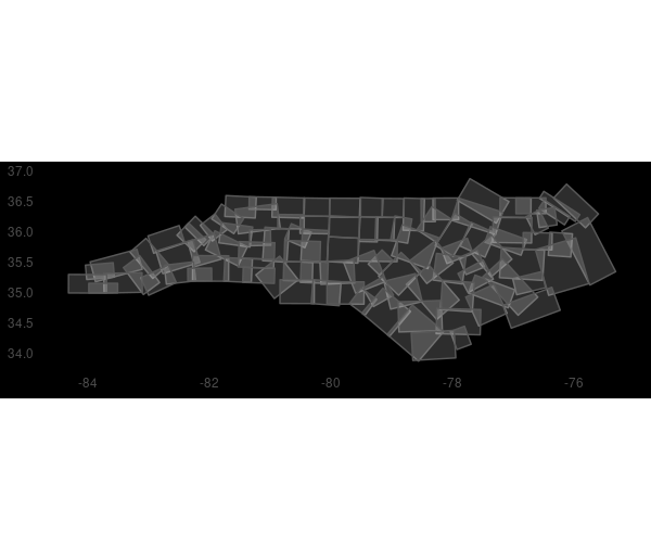
Plotting all the counties minimum bounding boxes together:

pmap_dfr(nc, min_box_sf) %>% 
  ggplot() +
  geom_sf(alpha = .2)

^{Created on 2021-08-20 by the reprex package (v2.0.1)}